Rhino: Bistatic Delay-Doppler Reference for Passive Radar Applications
The “Rhino” dataset comprises multiple bistatic radio channel measurements between one stationary transmitter and one stationary receiver recorded within a controlled environment. During the individual measurements, a target emulator rotates two metallic spheres, thereby creating two passive targets within the wireless channel. Since the position of transmitter, receiver, and both spheres have been recorded during the measurements, it is possible to calculate an analytical delay-Doppler ground truth for the multipath components of both spheres. Consequently, “Rhino” constitutes a benchmark for the objective and reproducible evaluation of delay-Doppler parameter estimation algorithms.
| Property | Value |
|---|---|
| Center Frequency | 5.9 GHz |
| Signal Type | Multi-Sinus |
| Symbol Duration | 64 us |
| Bandwidth | 160 MHz |
| Subcarriers | 1024 |
| Subcarrier Spacing | 156.25 kHz |
| Number of TXs | 1 |
| Number of RXs | 1 |
Introduction §
“Rhino” is part of a measurement campaign that took place in Ilmenau, Germany in February 2019. The measurements have been conducted in a controlled environment within the virtual road simulation and test area (VISTA) which is part of the Thüringer Innovationszentrum Mobilität (ThIMo). The goal of the campaign was to provide metrologically assessable SISO channel data that can be utilized to evaluate and benchmark delay-Doppler parameter estimation algorithms. Therefore, the measurement setup comprises two rotating spheres, resulting in two distinct propagation paths within the measured channel frequency responses. The “Rhino” datasets provides these channel frequency responses for a variety of bistatic measurement angles \(\delta\), covering forward, backward, and bistatic scattering scenarios. Consequently, the available data allows for the assessment of delay-Doppler parameter estimation algorithms under varying conditions, including changes in the ratio of Line-of-Sight (LoS) strength to target reflection strength, as well as the resolution of propagation paths that are below the Rayleigh limit.
Applications §
This dataset has a number of possible applications, for example
- the validation of radar algorithms in a controlled environment (passive target detection, tracking, and localization),
- the assessment of the high resolution capabilities of delay-Doppler estimation algorithms, or
- the performance comparison of different parameter estimation algorithms.
Getting Started §
The “Rhino” dataset is published and available for download [D1]. In addition, we provide a comprehensive documentation on our website [D2]. Once downloaded, use the Python snippets provided below to load and process the data.
Measurement Setup §
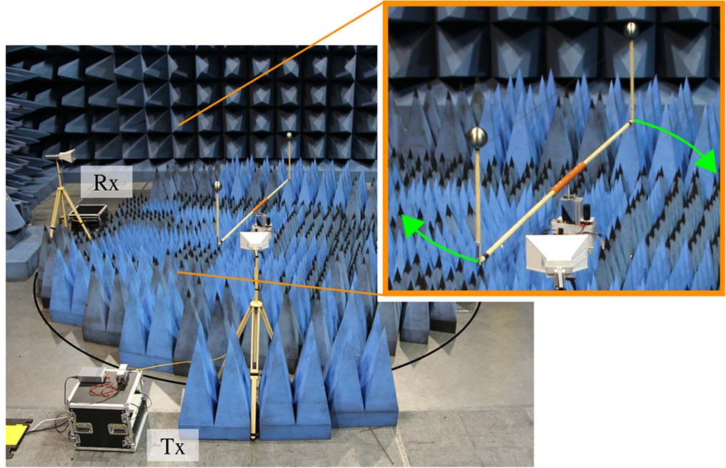
In [1], Schwind presents a detailed description of the measurement setup and some initial delay-Doppler parameter estimation results. In essence, two metallic spheres are mounted on a metal rod attached to a motor. The bistatic measurement angle \(\delta\) spans between the transmitter (TX), the motor, and the receiver (RX). In the dataset, this angle varies in ten-degree increments. As a result, the channel measurements include forward \((\delta \approx 180^\circ)\), backward \((\delta \approx 0^\circ)\), and bistatic scattering scenarios. Below you can find a schematic drawing of the setup.

By simultaneously recording channel frequency responses and the positions of the TX, RX, and both spheres, it is possible to calculate the analytical delay-Doppler parameters of both spheres. These values serve as ground truth in the corresponding delay-Doppler spectra, as shown in the following figure.

Data Format §
The following sections describe the structure of the dataset directory and the associated files.
Directory Structure §
The dataset has the following structure.
rhino/
├── results
│   ├── cfar
│   │   ├── Results_delta0.h5
│   │   ├── Results_delta10.h5
│   │   ├── Results_delta20.h5
│   │   └── ...
│   ├── deepest
│   │   ├── Results_delta0.h5
│   │   └── ...
│   └── pymax
│       ├── Results_delta0.h5
│       └── ...
├── Sphere_1
│   └── Data
│       ├── Info.json
│       └── Location.h5
├── Sphere_2
│   └── Data
│       ├── Info.json
│       └── Location.h5
└── Tx_0_to_Rx_0-350
    └── Data
        ├── FrequencyResponses.h5
        ├── LocationRx.h5
        └── LocationTx.h5
The subdirectory Tx_0_to_Rx_0-350/ comprises the measured channel frequency responses FrequencyResponses.h5 as well as the corresponding positions of the TX LocationTx.h5 and the RX LocationRx.h5.
Furthermore, Sphere_1/ and Sphere_2/ store the location information of the two passive targets in the Location.h5 files and some additional target-related meta information in the Info.json files.
In addition to the measurements, we provide our delay-Doppler parameter estimation results of the data within the results/ directory, utilizing three different algorithms, namely PyMax, DeepEst, and CFAR.
Each algorithm-specific subdirectory contains one file, Results_delta{delta}.h5, for each bistatic measurement angle \(\delta\).
The results are part of a measurement-based performance comparison of delay-Doppler parameter estimation algorithms.
Further information on the three algorithms and on how their results are used for comparison can be found in [2] and [3].
File Format §
We store the data within HDF5 files.
An abstract description of this file format can be found on our website [D3].
When working with HDF5 files, we found the h5ls command line tool extremly helpful.
This tool enables the generation of tree-like overviews of HDF5 files, presenting all relevant information, such as group and dataset names, dataset shapes, and available metadata.
Utilizing this information, it is easy to navigate the HDF5 file and load the desired data into memory.
The h5ls tool is available on the official HDF5 website and you can analyze an HDF5 file by invoking the following command.
h5ls -r h5_file.h5
The following sections introduce the three types of HDF5 files present in the “Rhino” dataset.
Frequency Response File §
The FrequencyResponses.h5 file has the following structure.
h5ls -r FrequencyResponses.h5
/                        Group
/FrequencyResponses      Group
/FrequencyResponses/Data Dataset {15600, 1024, 36}
/FrequencyResponses/MetaData Group
/FrequencyResponses/MetaData/Angle Group
/FrequencyResponses/MetaData/Angle/BistaticAngle Dataset {36}
/FrequencyResponses/MetaData/Frequency Group
/FrequencyResponses/MetaData/Frequency/Frequency Dataset {1024}
/FrequencyResponses/MetaData/Snapshot Group
/FrequencyResponses/MetaData/Snapshot/Index Dataset {15600}
/FrequencyResponses/MetaData/Snapshot/TimeStamp Dataset {15600}
The FrequencyResponses group comprises the channel frequency responses stored in the dataset Data.
This dataset has the shape \((15600 \times 1024 \times 36)\), corresponding to \((\text{Symbol Timestamp} \times \text{Subcarrier Frequency} \times \text{Bistatic Measurement Angle})\).
In addition, the MetaData group contains the physical values associated with these measurement dimensions.
Location Files §
The location files store the location of the TX, RX, and both spheres.
To this end, LocationTx.h5 file contains the position and orientation of the TX, which remained constant throughout the entire measurement campaign.
Consequently, all corresponding datasets contain only a single element.
h5ls -r LocationTx.h5
                        Group
/PoseData                Group
/PoseData/MetaData       Group
/PoseData/MetaData/Angle Group
/PoseData/MetaData/Angle/BistaticAngle Dataset {1}
/PoseData/PosX           Dataset {1}
/PoseData/PosY           Dataset {1}
/PoseData/PosZ           Dataset {1}
/PoseData/RotX           Dataset {1}
/PoseData/RotY           Dataset {1}
/PoseData/RotZ           Dataset {1}
The location of the RX did not change during a single measurement. However, it varied between measurements to create different bistatic measurement angles \(\delta\). Consequently, all HDF5 datasets contain one entry for each angle.
h5ls -r LocationRx.h5
/                        Group
/PoseData                Group
/PoseData/MetaData       Group
/PoseData/MetaData/Angle Group
/PoseData/MetaData/Angle/BistaticAngle Dataset {36}
/PoseData/PosX           Dataset {36}
/PoseData/PosY           Dataset {36}
/PoseData/PosZ           Dataset {36}
/PoseData/RotX           Dataset {36}
/PoseData/RotY           Dataset {36}
/PoseData/RotZ           Dataset {36}
In contrast, the positions of the spheres vary during a single measurement. The corresponding positions were recorded at the same sample rate as the frequency response symbols, resulting in \(15600\) positions. Since the trajectories of the spheres are similar across all measurements, the sphere positions do not depend on \(\delta\).
h5ls -r Location.h5
/                        Group
/PoseData                Group
/PoseData/MetaData       Group
/PoseData/MetaData/Snapshot Group
/PoseData/MetaData/Snapshot/Index Dataset {15600}
/PoseData/MetaData/Snapshot/TimeStamp Dataset {15600}
/PoseData/PosX           Dataset {15600}
/PoseData/PosY           Dataset {15600}
/PoseData/PosZ           Dataset {15600}
/PoseData/RotX           Dataset {15600}
/PoseData/RotY           Dataset {15600}
/PoseData/RotZ           Dataset {15600}
Result Files §
The result files store parameter estimation results derived from the measured frequency responses. In particular, we performed delay-Doppler estimation on non-overlapping frames of size \((100 \times 1024)\). Each frame thus comprises \(100\) frequency response symbols, resulting in \(156\) frames for the complete dataset.
h5ls -r Results_delta0.h5
/                        Group
/Results                 Group
/Results/Delay           Dataset {156}
/Results/Doppler         Dataset {156}
/Results/MetaData        Group
/Results/MetaData/Snapshot Group
/Results/MetaData/Snapshot/Index Dataset {156}
/Results/MetaData/Snapshot/TimeStamp Dataset {156}
/Results/PowGamma        Dataset {156}
/Results/dBGamma         Dataset {156}
The Snapshot group contains the index and timestamp of the first symbol of each frame.
For each frame, the results include a variable number of propagation paths, with each path characterized by a propagation delay, Doppler shift, and path power.
Loading any of these parameters returns a nested np.ndarray of one-dimensional np.ndarray’s.
Data Processing §
The following sections provide several introductory code snippets that demonstrate how to interact with the dataset.
Loading Channel Data §
The complex channel frequency response is stored as a compound datatype in the HDF5 dataset at /FrequencyResponses/Data.
Specifically, the fields real and imag represent the real and imaginary parts of the complex values, respectively.
The following Python function loads the snapshots for a specific bistatic measurement angle within the interval \([\text{start}, \text{stop})\).
import h5py as h5
import numpy as np

def load_complex_channel_data(file_path, sample_indices, bistatic_angle):
    """
    Loads complex channel data and associated axes.
    Arguments:
        file_path: str: Path to FrequencyResponses.h5 file
        sample_indices: Tuple[int, int]: A slice (start, stop) defining the
            slow-time (snapshot) samples to load from file.
        bistatic_angle: int: An integer in the range [0,35] defining the bistatic
            measurement angle \delta between transmitter and receiver.
    Returns:
        complex_data: np.ndarray: 2-D array (slow-time, frequency)
        ts: np.ndarray: array of timestamps [s] corresponding to the loaded samples
        ff: np.ndarray: array of subcarrier frequency values [Hz]
        aa: int: bistatic measurement angle \delta [deg]
    """
    sample_indices_slice = slice(sample_indices[0], sample_indices[1])
    timestamp_path = "/FrequencyResponses/MetaData/Snapshot/TimeStamp"
    frequencies_path = "/FrequencyResponses/MetaData/Frequency/Frequency"
    bistatic_angle_path = "FrequencyResponses/MetaData/Angle/BistaticAngle"

    with h5.File(file_path, "r") as f:
        # Read timestamp, frequency axes and compound dataset
        ts = f[timestamp_path][sample_indices_slice]
        ts_unitscaler = f[timestamp_path].attrs["UnitScaler"]

        ff = f[frequencies_path][:]
        ff_scaler = f[frequencies_path].attrs["UnitScaler"]

        aa = f[bistatic_angle_path][bistatic_angle]
        aa_scaler = f[bistatic_angle_path].attrs["UnitScaler"]

        data = f["/FrequencyResponses/Data"][
            sample_indices_slice, :, bistatic_angle
        ]

    complex_data = data["real"] + 1j * data["imag"]

    return (
        complex_data,
        ts * ts_unitscaler,
        ff * ff_scaler,
        aa * aa_scaler,
    )
Loading Position Data §
The following snippet loads the position information of the TX, RX, or a sphere.
import h5py as h5
import numpy as np

def load_position_data(file_path, sample_indices=None, bistatic_angle=None):
    """
    Loads position information of TX, RX, or target.
    Arguments:
        file_path: str: Path to the *.h5 location file
        sample_indices: Tuple[int, int]: A slice (start, stop) defining the
            slow-time (snapshot) samples to load from file.
        bistatic_angle: int: An integer in the range [0,35] defining the bistatic
            measurement angle \delta between transmitter and receiver.
    Returns:
        pos_arr: np.ndarray: 2-D array (slow_time, [x,y,z])
    """
    with h5.File(file_path, "r") as ff:
        # no time and angle given = TX Pos
        if sample_indices is None and bistatic_angle is None:
            x_pos = ff["PoseData/PosX"][:]
            y_pos = ff["PoseData/PosY"][:]
            z_pos = ff["PoseData/PosZ"][:]
            pos_arr = np.array(
                [x_pos, y_pos, z_pos], dtype=np.float64
            ).reshape((1, 3))
        # no time given = RX Pos
        elif sample_indices is None:
            x_pos = ff["PoseData/PosX"][bistatic_angle]
            y_pos = ff["PoseData/PosY"][bistatic_angle]
            z_pos = ff["PoseData/PosZ"][bistatic_angle]
            pos_arr = np.array(
                [x_pos, y_pos, z_pos], dtype=np.float64
            ).reshape((1, 3))
        # no angle given = Target Pos
        elif bistatic_angle is None:
            sample_indices_slice = slice(sample_indices[0], sample_indices[1])
            x_pos = ff["PoseData/PosX"][sample_indices_slice]
            y_pos = ff["PoseData/PosY"][sample_indices_slice]
            z_pos = ff["PoseData/PosZ"][sample_indices_slice]
            pos_arr = np.column_stack((x_pos, y_pos, z_pos))
        else:
            Exception("Unable to load position information!")
    return pos_arr
Calculating Ground Truth Parameters §
Calculating the bistatic delay and Doppler of a sphere requires the positions of the TX, RX, and the sphere. The following Python scripts demonstrate one approach to perform this calculation. Further information about the underlying formulas can be found in [1].
import h5py as h5
import numpy as np
import scipy as sc

def calc_position_vector(tx_pos, tar_pos, rx_pos):
    """
    Calculates the position vector between target-TX and target-RX.
    Arguments:
        tx_pos: np.ndarray: array of the TX position (fixed)
        tar_pos: np.ndarray: array of the target position
        rx_pos: np.ndarray: array of the RX position (fixed)
    Returns:
        tx_vec: np.ndarray: array of the position vector TX-target
        rx_vec: np.ndarray: array of the position vector target-RX
    """
    tx_vec = tx_pos - tar_pos
    rx_vec = rx_pos - tar_pos
    return tx_vec, rx_vec


def calc_delay(tx_vec, rx_vec):
    """
    Calculates the bistatic delay given target-TX and target-RX vectors. Returns
    the delay in the middle of the frame.
    Arguments:
        tx_vec: np.ndarray: array of position vector TX-target
        rx_vec: np.ndarray: array of position vector target-RX
    Returns:
        delay: float: Bistatic ground truth delay of the target
    """
    total_len = np.linalg.norm(tx_vec, axis=1) + np.linalg.norm(rx_vec, axis=1)
    delay = total_len / sc.constants.c
    # use middle of the frame for ground truth
    delay = delay[delay.shape[0] // 2]
    return delay


def calc_doppler(tar_pos, tx_vec, rx_vec, t_delta, lambda_c):
    """
    Calculates the bistatic Doppler given target-TX and target-RX vectors. Returns
    the Doppler in the middle of the frame.
    Arguments:
        tar_pos: np.ndarray: array of target position
        tx_vec: np.ndarray: array of position vector TX-target
        rx_vec: np.ndarray: array of position vector target-RX
        t_delta: float: symbol duration [s]
        lambda_c: float: carrier wavelength [m]
    Returns:
        doppler: float: Bistatic ground truth Doppler of the target
    """
    # finite differences to approximate velocity in (x,y,z)
    d_tar_pos = np.diff(tar_pos, n=1, axis=0)
    d_tar = d_tar_pos[d_tar_pos.shape[0] // 2]
    v_tar = d_tar / t_delta
    # use middle of the frame for ground truth
    tx_vec = tx_vec[tx_vec.shape[0] // 2]
    rx_vec = rx_vec[rx_vec.shape[0] // 2]
    # normalize vectors for projection
    tx_vec_norm = tx_vec / np.linalg.norm(tx_vec)
    rx_vec_norm = rx_vec / np.linalg.norm(rx_vec)
    # project v_tar onto the tx-tar and tar-rx vectors
    v_proj_tx = np.inner(v_tar, tx_vec_norm)
    v_proj_rx = np.inner(v_tar, rx_vec_norm)
    # total relative velocity
    v_tot = v_proj_tx + v_proj_rx
    # doppler
    doppler = v_tot / lambda_c
    return doppler
Plotting Delay-Doppler Spectra §
A common step in radar-like applications is the calculation of delay-Doppler spectra. The following Python script plots the magnitude of the delay-Doppler spectrum in dB and overlays ground truth delay-Doppler parameters of both spheres.
import matplotlib.pyplot as plt

##################### DEFINE PARAMETERS #########################
# bistatic angle index
bistatic_angle = 2
# starting index
start_idx = 2000
# frame size in number of elements
frame_size = 100
# frame indices
frame_indices = (start_idx, start_idx + frame_size)
# oversampling factor (zero padding for fft interpolation)
osf = 10

###################### DELAY-DOPPLER SPECTRUM ##################
# loaded complex_data has dims (slow-time, sub-carriers)
complex_data, ts, ff, aa = load_complex_channel_data(
    "rhino/Tx_0_to_Rx_0-350/Data/FrequencyResponses.h5",
    frame_indices,
    bistatic_angle,
)
ts_size = ts.shape[0]
ff_size = ff.shape[0]
# symbol duration
t_delta = ts[1] - ts[0]
# carrier wavelength
f_c = ff[ff.shape[0] // 2]
lambda_c = sc.constants.c / f_c

# transform slow-time to Doppler frequency
dd_map = np.fft.fftshift(np.fft.fft(complex_data, axis=0, n=osf * ts_size))
# trasnform sub-carriers to delay
dd_map = np.fft.ifft(np.fft.ifftshift(dd_map, axes=1), axis=1, n=osf * ff_size)
# transform to dB and normalize
dd_map = np.abs(dd_map) ** 2
dd_map = dd_map / np.max(dd_map)
dd_map_db = 10 * np.log10(dd_map)
# create axes for plotting
doppler_axis = np.fft.fftshift(np.fft.fftfreq(len(ts), d=(ts[1] - ts[0])))
delay_axis = np.fft.ifftshift(np.fft.fftfreq(len(ff), d=(ff[1] - ff[0])))
delay_axis = delay_axis - delay_axis.min()
doppler_axis += (doppler_axis[1] - doppler_axis[0]) / 2

########################### GROUND TRUTH #######################
# ground truth section
tx_path = "rhino/Tx_0_to_Rx_0-350/Data/LocationTx.h5"
rx_path = "rhino/Tx_0_to_Rx_0-350/Data/LocationRx.h5"
tar1_path = "rhino/Sphere_1/Data/Location.h5"
tar2_path = "rhino/Sphere_2/Data/Location.h5"

# load tx and rx pos (same for both spheres!)
tx_pos = load_position_data(tx_path)
rx_pos = load_position_data(rx_path, bistatic_angle=bistatic_angle)
# sphere 1 ground truth
tar1_pos = load_position_data(tar1_path, frame_indices)
tx1_vec, rx1_vec = calc_position_vector(tx_pos, tar1_pos, rx_pos)
tar1_delay = calc_delay(tx1_vec, rx1_vec)
tar1_doppler = calc_doppler(tar1_pos, tx1_vec, rx1_vec, t_delta, lambda_c)
# sphere 1 ground truth
tar2_pos = load_position_data(tar2_path, frame_indices)
tx2_vec, rx2_vec = calc_position_vector(tx_pos, tar2_pos, rx_pos)
tar2_delay = calc_delay(tx2_vec, rx2_vec)
tar2_doppler = calc_doppler(tar2_pos, tx2_vec, rx2_vec, t_delta, lambda_c)

############################## VISUALIZATION ##########################
plt.figure(figsize=(8, 6))
# plot dd spectrum
plt.imshow(
    dd_map_db.T,  # .T so that Doppler is the horizontal axis
    extent=[doppler_axis[0], doppler_axis[-1], delay_axis[0], delay_axis[-1]],
    aspect="auto",
    vmax=0,
    vmin=-60,
    origin="lower",
)
plt.colorbar(label="Normalized Power (dB)")
# plot ground truth
plt.scatter(
    tar1_doppler,
    tar1_delay,
    marker="o",
    facecolors="none",
    edgecolors="red",
    linewidths=3,
    zorder=1,
    s=100,
    label="Sphere_1",
)
plt.scatter(
    tar2_doppler,
    tar2_delay,
    marker="o",
    facecolors="none",
    edgecolors="black",
    linewidths=3,
    zorder=1,
    s=100,
    label="Sphere_2",
)
plt.xlabel("Delay (s)")
plt.ylabel("Doppler Frequency (Hz)")
plt.title("Delay-Doppler Spectrum")
# limit for better visibility
plt.xlim([-2000, 2000])
plt.ylim([0, 200e-9])
plt.legend()
plt.show()
Executing the above snippet produces the following delay-Doppler spectrum.

References §
Dataset and Documentation §
- [D1] L. Mohr, M. Döbereiner, C. Andrich, A. Schwind, C. Schneider, and R. Thomä, “Rhino: Bistatic Delay-Doppler Reference for Passive Radar Applications,” Jan. 15, 2026. DOI:10.71758/refodat.72.
- [D2] “Rhino: Bistatic Delay-Doppler Reference for Passive Radar Applications,” EMS TU Ilmenau. [Online]
- [D3] “Abstract Specification,” EMS TU Ilmenau. [Online]
Related Publications §
- [1] A. Schwind, M. Döbereiner, C. Andrich, P. Wendland, G. Del Galdo, G. Schäfer, R. S. Thomä, and M. A. Hein, “Bi‑static delay‑Doppler reference for cooperative passive vehicle‑to‑X radar applications,” IET Microwaves, Antennas & Propagation, vol. 14, no. 14, pp. 1749–1757, 2020. DOI: 10.1049/iet‑map.2019.0991
- [2] L. Mohr, “Measurement-Based Performance Analysis of RADAR Estimation Algorithms,” 2024. DOI: 10.22032/dbt.63482
- [3] L. Mohr, M. Döbereiner, S. Schieler, J. Robert, C. Schneider, S. Semper, and R. S. Thomä, “Performance Comparison of Joint Delay‑Doppler Estimation Algorithms,” Oct. 2025. DOI: 10.48550/arXiv.2510.16200
Citation §
If you use this dataset, please cite the following data record.
@dataset{2026_rhino_dataset_Mohr,
  author = 	{Mohr, Lorenz
		and D{\"o}bereiner, Michael
		and Andrich, Carsten
		and Schwind, Andreas
		and Schneider, Christian
		and Thom{\"a}, Reiner},
  title = 	{{Rhino: Bistatic Delay-Doppler Reference for Passive Radar Applications}},
  year = 	{2026},
  month = 	{Jan},
  day =     {15},
  keywords = 	{Wireless Communication; Passive Radar; Channel Sounding; Delay-Doppler Estimation; Reference Dataset; Benchmark; sub-6-GHz measurements},
  doi =     {10.71758/refodat.72},
  url = 	{https://refodat.de/receive/refodat_mods_00000072},
  language = 	{en}
}